XTomo-LM 3

2D Tomography System with Tools for Layered Model Study

The third version of XTomo-LM solves almost all problems that had been posed in the beginning of the product's long history. Technically, the third version is adjusted to the present state of the x86/Windows platform – multicore processors, hyper-threading technology and last versions of the operating system. In XTomo-LM 3, tomography tools are immersed in the context of layered model kinematic interpretation. This makes it possible to apply tomography inversion to observations of waves of different types. The traditional first arrival tomography exists in this context as a special case.

Application Area

During its life cycle XTomo-LM was applied for data processing in different seismic investigations: CMP profiling, deep seismic soundings, wide-angle reflection and refraction profiling, various geological engineering surveys, borehole studies. Among XTomo-LM or XTomo-LM + DPU licensees there are exploration and servicing companies, geotechnical firms, research institutes and universities. Mostly, they are residents of Russian Federation; some are in Kazakhstan, Georgia, Italy and India.

About  XTomo-LM

Model representation

Model is described by a set of velocity values defined at nodes of a curvilinear mesh, which is formed by a set of verticals and a family of simple non-intersecting curves. Such mesh suits well to representing subhorizontal seismic boundaries  and some geological structures (fig. 1).

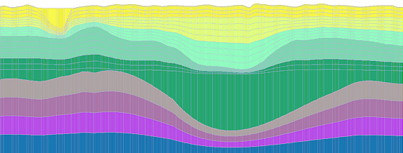Fig. 1. This layered model is represented exactly by a grid of the class described.

 

In modeling projects, the model wireframe – a set of seismic horizons – is known a priori. Each horizon can be imported from an ASCII file or drawn by the user in model editor. Then the horizon curve is automatically implanted into the existing mesh (possible, rectangle) and turns into one of its quasi-horizontal coordinate lines. The advantage of the curvilinear mesh and the XTomo-LM method of ray-tracing lies in that no special description of seismic boundaries is required. In inversion projects seismic horizons are imported either as priory information or as a result of interpretation by built-in or external tools.

 

Model Editor

The graphic model editor help perform three basic tasks: (1) change number of lines in a model subdomain; (2) change velocity in cells of a subgrid; and (3) change model geometry. The latter is implemented by changing one of quasi-horizontal lines in curve editor, which provided with the easy-to-use  user interface for pointwise editing, enforced by means of interpolation, approximation, and smoothing tools. Modifying line profile affects lines around it, but only in the limits defined by the user.

 

Forward problem (modeling)

Kinematic forward problem is posed for given source-receiver configuration (observation system) and given set of waves. The latter can include diving wave or/and reflections or/and head waves. Reflected and head waves are attached to seismic horizons. Solution of forward problem includes ray picture and traveltimes along rays represented as common source point traveltime curves. When observation system is dense, the picture contains too many rays to be informative. That's why XTomo-LM allows creating and visualizing ray samples. A ray sample is defined by subsets of sources, receivers and waves and even a model subdomain which rays must intersect. In inversion projects, forward problem solution, additionally, contains absolute and relative traveltime residuals, while ray sampling condition can include residual range. An example of a ray sample is shown on fig. 2.Traveltime curves can be viewed in the same or separate window; in case of inversion project observed traveltimes can be displayed together with the computed.

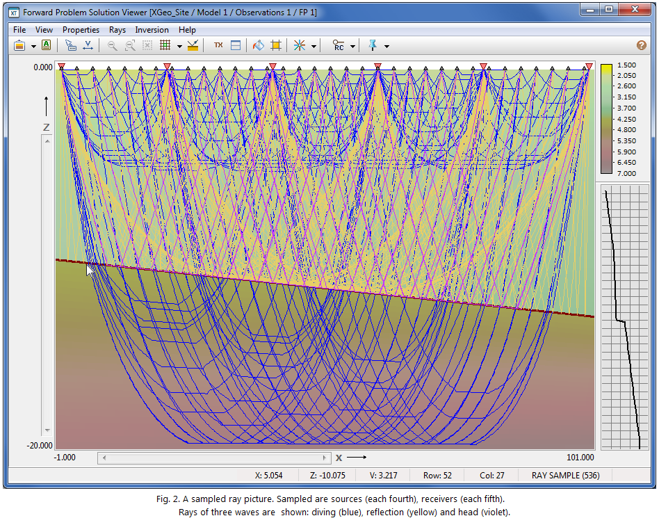
In inversion projects, ray picture analysis is of crucial importance. XTomo-LM has means of statistical analysis of ray samples and can build maps of ray coverage.  Ray coverage is a function of a grid cell equal to a number of rays (or subvertical rays, or subhorizontal rays) passing through a cell (fig. 3).  Ray coverage defines reliability of tomography inversion result: it is high for cells intersected by many rays in different directions and low for cells passed through by small number of rays. Ray coverage is akin to sensitivity for tomography inversion.

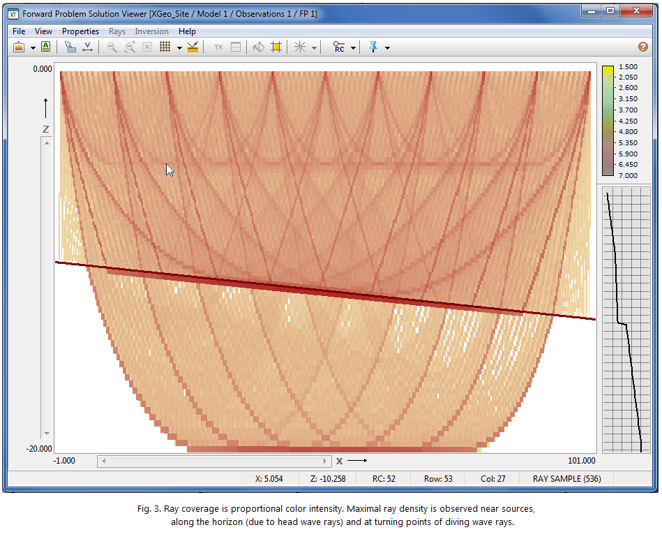
XTomo-LM forward problem allows modeling of converted waves too. The user has to define conversion coefficients for the boundary on which conversion takes place and those located above it.

Forward problem pertains to "heavy" computations and requires maximum of system resources. In version 3, ray-tracing for each source is performed by one logical processor. For systems with many logical processors computation time drops drastically. For example, for dense grids and large number of rays a system with 8 logical processors solves the problem 3.6 times faster than a system with 2 processors.

 

Inverse Problems

XTomo-LM is designed for solving inverse problems of two classes. The first class includes seismic tomography problems. The second class includes time-distance curve inversion problems (TX curves of different waves are supposed to be extracted from 2D profiling data). The inversion problems are stated with relevant mathematical rigor in the documentation. The original algorithms for getting solutions are developed with special care for their robustness.

 

Tomography Inversion

Tomography inversion refines initial velocity by minimizing residuals between the observed times and the times computed by solving forward problem for initial model. Traveltimes of different waves can take part in this procedure, first arrival timess, in particular. The latter are treated as arrival times of transient or diving wave.  XTomo-LM allows doing tomography for ray samples from forward problem solution as well. For example, it is possible to do that for rays of the reflection from a layer floor and add to them rays of diving wave with turning points within the layer. At that, velocity in above layers can be frozen. Thus, tomography on ray samples can be regarded as a means of layer-by-layer interpretation. Of course, the latter is not formalized. The result of inversion can be viewed on the difference map (fig. 4).

 

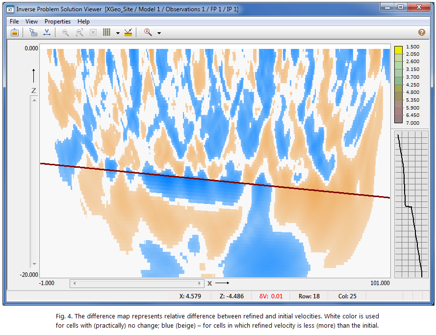
TX-curve Inversion

The first problem of this type is inversion of diving wave traveltimes for getting velocity distribution. The method used is based on a well-posed one-dimensional inverse problem for one TX-curve. The problem solution can be found with a stable algorithm. Applied to an appropriate sample of travel-curves observed on the line, the algorithm allows building a two-dimensional velocity distribution belonging to the class of functions increasing in depth at each line point. The function bult can be used as a good initial approximation for tomography inversion.

In reconstruction of a reflectors (refractor) from the reflection (head wave) traveltime curves, the velocity in the overburden is supposed to be a known function. The robust reconstruction is possible under the assumption that the velocity is vertically constant in a strip around the horizon. This area can be very roughly estimated practically always. Replacing the given velocity with a constant in the strip we get the first approximation of the solution using the base algorithm. Then applying a curvilinear grid technique, we reduce the strip thickness practically to zero in one or two iterations.

 

Environment

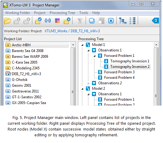
Inversion of observed data is multi-step process even in the simplest case of first arrival tomography. The reason is that linearization of non-linear problem of minimization of time residuals can be carried out under the assumption of small velocity variations. Consequently, refinement of the initial velocity moves on by small steps.  That implies that the processing system must store intermediate data and enable the user to view and analyze them. In XTomo-LM this task is carried out by the system head program – Project Manager (fig. 5).  The project data are represented in the form of four-level tree. Root nodes store successive versions of the model obtained by direct editing or by tomography inversion; second-level nodes store information on the observation system; then go nodes for forward problem solutions and for tomography inversion results. Then a new interpretation cycle begins. The tree represents also different interpretation paths, initiated by different samples of initial data, different ray samples or different program adjustments.

Work with ASCII files with description of observation systems is an important part of the environment. For interpretation problems such files contain IDs and coordinates of sources and receivers as well as traveltimes for all waves observed. For modeling problems they contain only positional data.  Import and verification of  observation files  is carried out by the special component called SRT Port.  It supports a data warehouse in which the verified content of each observation file is stored as a database ready for repeated use.  Data samples from such databases are used as input data for inversion or modeling tasks. 

 

Export

At every step of processing the user can export data to graphic and text files. Graphic export allows getting most part of screen images (models, ray pictures and so on) in graphic files with scale, axis and headings adjusted by the user. Text export makes the system open for applying other interpretation tools and for getting high-quality maps and pictures in presentation graphic systems.

XTomo-LM has English user interface and is delivered with documentation and context help system in English or Russian.